understand the basic assumptions of predictive analytics.
be familiar with the kinds of statistical approaches that are most commonly used in predictive analytics.
be able to conduct predictive analytics within R.
Note
The material in this section, and that in the following section on Prescriptive Analytics, may be quite challenging. Don’t worry - we’ll cover it in more detail in the Research Methods module in Semester Two. However, it’s useful at this stage to gain a general familiarity with some of the concepts below, even if you don’t fully understand them at this point.
18.2 Introduction
‘Predictive analytics’ describes the use of data analysis to make predictions about the future, based on data that we already have.
Predictive analytics are useful in a variety of different contexts within sport. For example:
They can help optimise the performance of athletes by predicting physical and mental readiness, thereby enabling personalised training schedules and tactics. They can help us understand an athlete’s strengths, weaknesses, and the areas they need to work on.
Through predictive analytics, teams can identify patterns and trends related to injuries. This can help in predicting potential injuries before they occur, enabling preventative measures, timely interventions, and thus reducing player downtime.
Predictive models can analyse a vast amount of player performance data to identify rising stars or undervalued players. It helps teams in their recruitment process by providing data-driven insights into potential fits for the team’s strategy and structure.
Predictive analytics can be used to model possible game scenarios based on past performance data of teams and players. This can help coaches and strategists to design game plans, make real-time decisions, and adapt strategies for upcoming matches.
Predictive analytics can predict fan behaviour, preferences, and purchasing habits. This can help sports organisations to target marketing strategies, enhance fan engagement, improve ticket sales, and thus increase revenue.
18.3 What are ‘Predictive Analytics’?
18.3.1 Definitions
As noted above, the concept of predictive analytics describes a data-driven approach to making predictions. Predictive analytics uses existing data (i.e. data from events that have already happened) to make predictions about events that will (or may) occur in the future.
Predictive analytics use various modelling techniques such as regression, classification, clustering, and time series analysis to make predictions about the future. The type of technique used depends on the nature of the problem and the type of data available. We’ll learn more about these techniques towards the end of this module, and in the B1705 module in Semester 2.
A key assumption of predictive models is that they improve over time as they are trained with more and more data. In other words, they learn from the past to predict the future more accurately.
The more information we have about the past, the better we can predict the future (in theory).
It’s important to note that forecasting future events isn’t, of itself, particularly useful. One of the main goals of predictive analytics is to provide actionable insights. These insights allow organisations (and individuals, such as coaches) to make better decisions about current strategies, to mitigate risk, and to make the most of events that have still to happen.
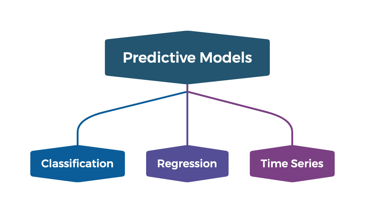
18.3.2 Three Types of Predictive Models
There are three main categories of predictive models that you are likely to encounter within sport data analytics. The following is a brief introduction to each, and really just scratches the surface. We’ll cover these in more greater detail in the Research Methods module in Semester 2 (B1705).
18.3.2.1 Type 1: Classification Models
‘Classification models’ are used to predict categorical or discrete output variables, often called ‘class labels’. We use them when the outcome of our predictive model is a binary or multi-class category, such as ‘yes’ or ‘no’, ‘win’ or ‘loss’, or ‘high risk’, ‘medium risk’, or ‘low risk’.
Building a classification model involves training the model on a dataset where the class labels are already known. This enables the model to ‘learn’ patterns or relationships between features and the class labels (which you might think of as ‘outcomes’). After training, the model is then used to predict the class labels of new, unseen data.
Various techniques are used to build classification models, including Logistic Regression, Decision Trees, Random Forests, Support Vector Machines, and Neural Networks. Each has its strengths and weaknesses, and the choice of technique depends on the nature of the data we’re working with, and the specific requirements of our prediction task.
In sport data analytics, classification models can be used in any situation with a binary or categorical outcome; for example, to predict whether a team will win, lose or draw a match, whether a player will be injured or not in the next game, or to categorise players into different performance groups (e.g. excellent, satisfactory, unsatisfactory).
18.3.2.2 Type 2: Regression Models
While classification models are useful when the predicted outcome is binary or categorical, regression models are used to to make predictions on continuous outcomes.
Regression analysis tries to estimate the relationships among a number of variables. It’s usually focussed on the relationship between a dependent variable (also known as the ‘outcome’ or ‘response’ variable) and one or more independent variables (often termed ‘predictors’, ‘covariates’, or ‘features’).
There are various types of regression models, including:
Linear Regression - the most basic type of regression where the relationship between the dependent and independent variables is assumed to be linear. It’s used when the outcome variable is continuous in nature, like predicting house prices or a player’s total season points.
Logistic Regression - used when the dependent variable is binary or dichotomous (having two outcomes, like win/lose or pass/fail). It provides the probability of a certain event occurring.
Polynomial Regression - used when the relationship between the independent and dependent variable is nonlinear. It involves transforming the independent variables to higher degrees and then running a linear regression on the transformed variables.
Multivariate Regression - when there are multiple independent variables that might influence the outcome, multivariate regression is used. It helps in understanding which variables have the most significant impact on the outcome and how these variables interact with each other.
In sport data analytics, regression models can be used to predict a wide range of outcomes, such as a team’s likely score in a match, a player’s future performance based on past statistics, or the probability of an injury based on training load data.
18.3.2.3 Type 3: Time Series Models
Time series modeling is a statistical method used to analyse time-ordered data points, typically collected at consistent intervals. The primary goal is to predict future values based on historical trends and patterns.
We’ll cover time series analysis in much more detail during B1705 in Semester Two.
The most common time series models you’ll encounter are:
Autoregressive (AR) Models: These models use the relationship between an observation and a number of lagged observations (previous time periods).
Moving Average (MA) Models: Instead of using past values of the forecast variable in a regression-like fashion, MA models use past forecast errors in a regression-like model.
Autoregressive Integrated Moving Average (ARIMA) Models: Combining AR and MA models, ARIMA also accounts for differencing the series to make it stationary (i.e., data values have consistent statistical properties over time).
Seasonal Decomposition of Time Series (STL): This method decomposes a series into seasonal, trend, and residual components.
Exponential Smoothing (ETS) Models: These models weigh past observations with exponentially decreasing weights to forecast future data points.
Because a lot of sport data is time-based, time series models are useful in lots of different sport data analytics scenarios. For example, you may wish to
predict how a player’s performance might change over the course of a season or their career
forecast a player’s batting average or points-per-game over time.
track and predict recovery timelines for athletes. By analysing the time series data of an athlete’s rehabilitation metrics (e.g., range of motion, strength levels), one can better estimate when an athlete might return to play.
Because they take ‘seasonality’ into account, they’re useful for situations were you want to identify patterns where teams or players might have seasonal peaks or troughs.
18.4 Using R for Predictive Analytics
As you’d expect, R offers a wide range of libraries for predictive analysis.
Here are some of the most useful (we’ll return to some of these in Semester 2):
caret: This package provides a consistent interface for training and tuning a wide variety of machine learning models. It simplifies (!) the process of creating complex predictive models.
randomForest: As the name suggests, this package is used to create random forest models, which are powerful ensemble methods for classification and regression.
rpart and party: These packages are useful for creating decision tree models. rpart stands for Recursive Partitioning and Regression Trees, while party stands for A Laboratory for Recursive Partitioning.
e1071: This package contains functions for statistics and probability theory, which includes SVM (Support Vector Machine) classifier and Naive Bayes classifier.
glmnet: This package is used for regression with penalized estimation, providing capabilities to perform ridge regression and lasso.
gbm: This package implements generalised boosted regression models, a flexible class of ensemble learning methods.
xgboost: An implementation of the gradient boosting framework, this package is known for its speed and performance.
forecast: This package is particularly useful for time series forecasting, offering methods like ARIMA, exponential smoothing, and more.
18.5 Data Preparation in R for Predictive Analytics
By this point, you should be familiar with all the steps necessary to import, clean and prepare your data for analysis. However, there are some additional steps we often need (or wish) to take prior to engaging in predictive analysis.
18.5.1 Data Transformation: Scaling, Encoding
Data transformation is a crucial step in your predictive analysis pipeline. It involves converting your raw data into a format that is suitable for modeling. In the following sections, we’ll focus on two common types of data transformation: scaling and encoding.
18.5.1.1 Scaling
Scaling is used to standardise the range of continuous or integer variables. The goal is to make sure different features have similar scales so that they contribute equally to the model. Without scaling, features with larger ranges may dominate the model.
Note
Imagine you’re exploring how to predict a basketball player’s performance based on multiple features like their height, weight, minutes played, and points scored per game.
Consider the following features in a dataset:
Height (in centimeters): Typically between 170 cm and 220 cm
Weight (in kilograms): Typically between 60 kg and 130 kg
Minutes played per game: Typically between 0 and 48
Points scored per game: Typically between 0 and 30
These features vary significantly in scale. Without scaling, a machine learning model (e.g., a regression or a neural network) may give undue importance to features with larger values (like height and weight) simply because they dominate the numerical space, leading to biased predictions.
By scaling the data, all features are brought to a common range, allowing the model to consider each feature’s relative importance more fairly.
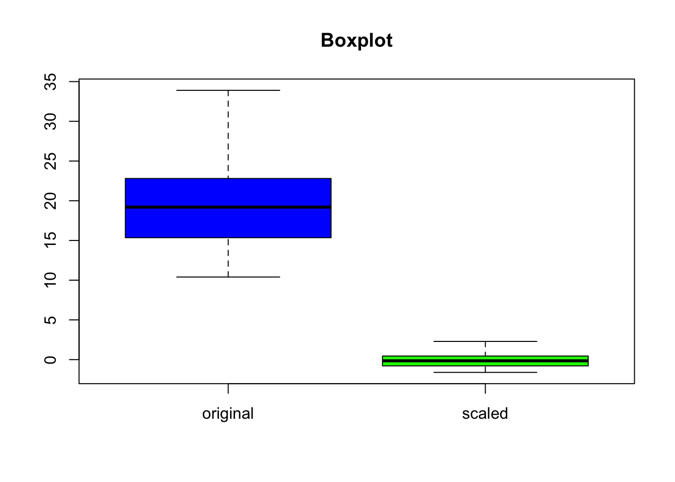
For scaling, we can use the scale function in R, which performs standardisation (subtracting the mean and dividing by the standard deviation).
Let’s assume we’re working with the [mtcars] dataset, and we want to scale the mpg (miles per gallon) feature.
rm(list =ls()) ## create a clean environment# load the mtcars datasetdata(mtcars)# apply the scale functionmtcars$mpg_scaled <-scale(mtcars$mpg)# we can see the difference in a boxplot between the unscaled and the scaled databoxplot(mtcars$mpg, mtcars$mpg_scaled, main="Boxplot",names=c("original", "scaled"), col=c("blue", "green"))
Scaling data ensures that different features or variables have a standard scale, making it easier for algorithms, especially those sensitive to feature magnitudes like gradient descent and k-means clustering, to converge faster and perform optimally.
By scaling data, we also prevent variables with larger scales from dominating models, thereby ensuring that all features contribute equally to the model’s performance.
You may be wondering how to decide whether or not to scale your data. There is no definitive answer to this. However, some things you will want to consider (in the context of predictive modelling) are:
Algorithm sensitivity: As we’ll learn in B1705, distance-based algorithms like K-means clustering or K-nearest neighbours are affected by the magnitude of variables. Unscaled data can result in larger scale variables unduly influencing the outcome. Gradient-based optimisation algorithms, such as those used in many machine learning models (like neural networks, logistic regression, and SVM with certain kernels), can also converge faster with scaled data.
Interpretability: In algorithms like linear regression, scaling can affect the interpretability of coefficients. Unscaled data allows us to directly interpret the coefficients in terms of the original units rather than trying to remember which features in our data are ‘bigger’ than others in terms of scale.
Data distribution & outliers: If our data has many outliers, robust scaling methods might be preferred over standard methods like min-max scaling. If our features have significantly different ranges, scaling might be necessary to ensure balanced contributions from all features.
Domain knowledge & context: In some cases, the real-world meaning of a variable’s magnitude is essential for the model’s accuracy or interpretability. For example, consider the case of height and BMI (Body Mass Index):
Height is a direct measure of a person’s stature, and its actual value carries a lot of meaning. For example, in sport, height can be a key predictor of performance in certain positions (e.g., basketball or volleyball players). The absolute magnitude of height is crucial, and scaling it could distort the real-world relationships.
BMI is calculated using both height and weight as it involves a specific formula \(BMI=\frac{\text{weight (kg)}}{\text{height (m)}^2}\). Here, the actual values of height and weight must remain unscaled because the formula requires them in their specific units. Scaling either variable could render the BMI calculation meaningless, as it relies on actual physical dimensions.
Similarly, in some physiological models, the raw units matter because they are tied to human health, performance metrics, or limitations. For instance:
VO2 max (maximum oxygen consumption) or heart rate are often used in sports analytics, particularly in endurance sports like running or cycling. These values are physiologically significant in their actual scales. Scaling might obscure their real-world relevance because slight changes in these metrics can have large, direct impacts on an athlete’s performance and health.
Computational constraints: Scaling can sometimes aid in speeding up the computational process, especially in models where matrix computations are intensive.
18.5.1.2 Encoding
‘Encoding’ is used to convert categorical variables into a format that can be used by machine learning algorithms. Most commonly, we would use ‘one-hot encoding’.
Note
One-hot encoding is a method used to convert categorical variables into a binary format, where each unique category is represented by a separate column with values of 0 or 1. This technique prevents machine learning models from assuming any ordinal relationship between categories and makes categorical data usable in algorithms that require numerical inputs. So for example, if a player is a forward, they’d be encoded 1 under forward, and 0 under midfielder and 0 under defender.
For encoding, I suggest you use the model.matrix function in R.
Let’s encode the [cyl] (number of cylinders) feature in the mtcars dataset.
# we will apply one-hot encoding using model.matrixencoded_cyl <-model.matrix(~as.factor(mtcars$cyl)-1)# now, we convert the matrix to a data frame and add it to the original datamtcars <-cbind(mtcars, as.data.frame(encoded_cyl))head(mtcars)
In the model.matrix function, the -1 removes the intercept column, which is not needed for one-hot encoding.
18.5.1.3 Why Is this important?
This might all seem quite challenging, and you may be wondering why we would wish to complicate things.
Scaling and encoding are important pre-processing steps that can significantly impact the performance of predictive models. Many of these techniques are only really required when you’re dealing with very large datasets - for example those generated by real-time capture of physiological data during a rugby match for multiple players.
Remember, important decisions are often made on the basis of predictive models, and we want to get them right!
Perhaps most importantly, scaling ensures that all features contribute equally to the model. Without scaling, features with larger scales might unduly influence the model, even if they’re not necessarily more important.
Encoding, on the other hand, allows you to use categorical data in predictive models. Many machine learning algorithms require numerical input and can’t work with categorical data directly. Encoding transforms these categorical variables into a suitable numerical format.
Keep in mind that these transformations should be applied with care, and the transformed data should always be examined to ensure that the transformations have been applied correctly.
18.5.2 Splitting Data into Training and Test Sets
When building a predictive model, we need to evaluate the performance of our model not just on the data it was trained on, but also on unseen data. This helps us to evaluate how well our model generalises to new data, which is a key aspect of its predictive power.
To do this, we usually split our dataset into two parts: a training set and a test set. The model is trained on the training set and then evaluated on the test set.
18.5.2.1 Doing this in R
Step 1: Load Required Library
First, we need to install and load the caret library which provides the createDataPartition function for splitting data.
Tip
In the following code I’ve used a command that lets you check whether a required package is installed or not. This can be useful if you’re passing your code to other people, or working on different computers.
# Install the caret package if not installedif(!require(caret)) install.packages('caret')
Loading required package: caret
Loading required package: ggplot2
Loading required package: lattice
# Load the caret packagelibrary(caret)
Step 2: Load Your Data
For this example, we’ll use the built-in mtcars dataset. You can replace this with your own dataset.
# Load the mtcars datasetdata(mtcars)
Step 3: Split the Data
Now, we’ll split the data into a training set and a test set. We’ll use 70% of the data for training and 30% for testing.
# Set the seed for reproducibilityset.seed(123)# Create the data partitiontrainIndex <-createDataPartition(mtcars$mpg, p = .7, list =FALSE)# Create the training settrainSet <- mtcars[trainIndex, ]# Create the test settestSet <- mtcars[-trainIndex, ]
The createDataPartition function generates indices based on stratified sampling, which helps to ensure that the training and test sets have similar data distributions.
The p = .7 argument specifies that 70% of the data should be used for training, leaving 30% for testing.
18.5.2.2 Why Is This Important?
Splitting data into ‘training’ and ‘test’ sets is a fundamental practice in machine learning and predictive analytics. It allows us to estimate the performance of your model on unseen data, which is a better indicator of the model’s effectiveness than its performance on the training data.
It also helps to detect overfitting, a common problem where the model performs well on the training data, but poorly on new, unseen data (and doesn’t give a great impression!).
If a model’s performance is much worse on the test set than on the training set, it may be overfitting the training data and failing to generalize well to new data.
Remember, it’s essential to only use the test set for evaluation purposes and not include it in any part of the model training process. Doing so could lead to optimistic bias in the estimated performance of the model.
18.6 Building Predictive Models in R
18.6.1 Linear Regression: Predicting Continuous Outcomes
Linear regression predicts a continuous response variable (such as a score or time) based on one or more predictor variables. In sport, for instance, you might want to predict a player’s total season points based on their training hours and previous season points.
For example, using a hypothetical dataset [player_data], we might want to predict [total_points] based on [training_hours] and [previous_points].
# First we load the dataset.url <-"https://www.dropbox.com/scl/fi/72x6r85ncsqn4hf1oszlm/t15_data_b1700_02.csv?rlkey=w9bakm4od1vi5vem1opyu69fp&dl=1"df <-read.csv(url)rm(url)
Call:
lm(formula = total_points ~ training_hours + previous_points,
    data = df)

Residuals:
    Min      1Q  Median      3Q     Max
-98.404 -43.841  -0.469  45.185  99.728

Coefficients:
                 Estimate Std. Error t value Pr(>|t|)
(Intercept)     122.88847    9.58659  12.819   <2e-16 ***
training_hours   -0.15074    0.24120  -0.625   0.5323
previous_points  -0.07742    0.03818  -2.028   0.0432 *
---
Signif. codes:  0 '***' 0.001 '**' 0.01 '*' 0.05 '.' 0.1 ' ' 1

Residual standard error: 53.26 on 457 degrees of freedom
Multiple R-squared:  0.009675,  Adjusted R-squared:  0.005341
F-statistic: 2.232 on 2 and 457 DF,  p-value: 0.1085
To build our model, I used the lm() function. The summary() function allows us to evaluate our model by inspecting the coefficients, R-squared, and p-values.
When interpreting our model, the coefficients represent the change in the response for a one-unit change in the predictor. The R-squared value indicates how well the model fits the data.
Logistic regression predicts the probability of a binary outcome. In sport, this could be predicting whether a team wins (1) or loses (0) based on certain features.
Example: Predicting match_outcome (win=1, lose=0) based on team_strength and opponent_strength.
# First we load the dataseturl <-"https://www.dropbox.com/scl/fi/g58fadnr4etjqgfyn1thl/t15_data_b1700_01.csv?rlkey=nb8hz1p4613tmucclafl4gyhv&dl=1"df <-read.csv(url)rm(url)
Call:
glm(formula = outcome ~ team_strength + opponent_strength, family = binomial(link = "logit"),
    data = df)

Coefficients:
                    Estimate Std. Error z value Pr(>|z|)
(Intercept)        0.2734007  0.2768076   0.988    0.323
team_strength     -0.0006983  0.0137504  -0.051    0.959
opponent_strength -0.0207486  0.0144327  -1.438    0.151

(Dispersion parameter for binomial family taken to be 1)

    Null deviance: 637.66  on 459  degrees of freedom
Residual deviance: 635.55  on 457  degrees of freedom
AIC: 641.55

Number of Fisher Scoring iterations: 3
To build our model, we use the glm() function with family=binomial(link='logit'). The summary() function provides coefficients, z-values, and p-values.
When interpreting our model, the coefficients show the log odds. You can convert them to odds ratios using the exp() function.
18.6.3 Time Series Forecasting: Predicting Future Trends
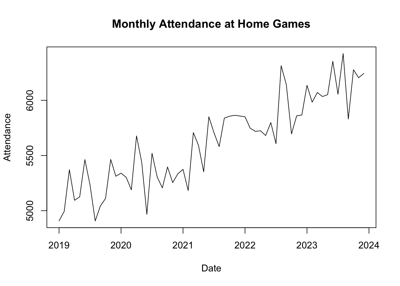
Time series forecasting predicts future values based on past patterns. In sport, this might involve forecasting spectator attendance at future games based on historical data.
The following dataset contains monthly attendance at home games over a period of five years:
# First we load the dataseturl <-"https://www.dropbox.com/scl/fi/8o1iwbrmdnxk2nsswzlj3/t15_data_b1700_03.csv?rlkey=ckf4o5vylblvyzd82lxvxc29n&dl=1"df <-read.csv(url)rm(url)
# Create a time series objectdf$attendance_ts <-ts(df$attendance, start =c(2019, 1), frequency =12)
# Plot the time series dataplot(df$attendance_ts, main ="Monthly Attendance at Home Games", xlab ="Date", ylab ="Attendance")
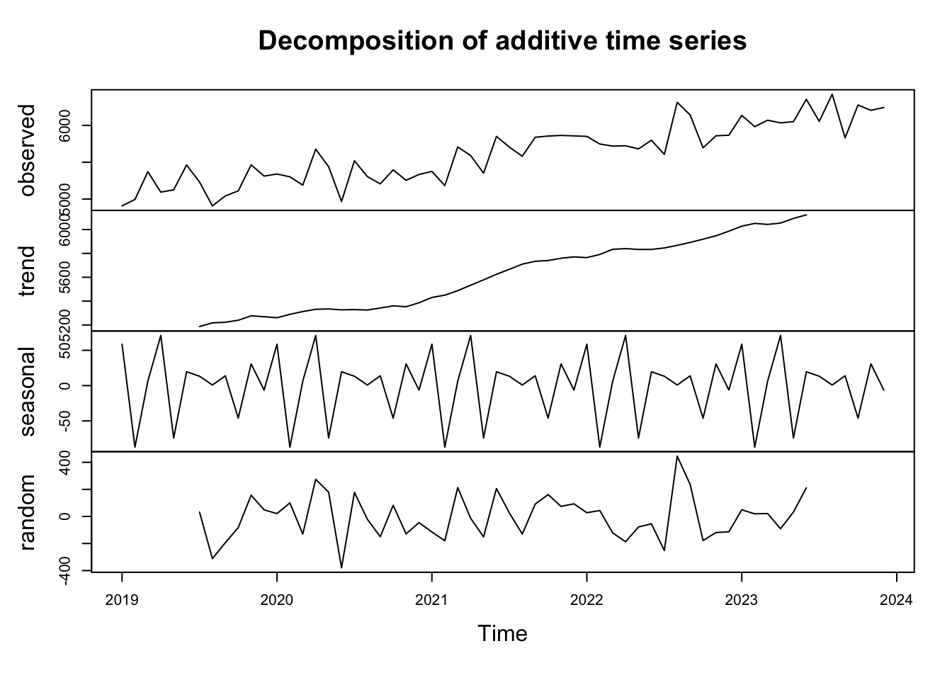
18.6.3.1 Time Series Decomposition
Before forecasting, it’s often useful to decompose the time series into its constituent components: trend, seasonality, and noise.
# Decompose the time seriesdecomposed_attendance <-decompose(df$attendance_ts)
# Plot the decomposed time seriesplot(decomposed_attendance)
18.6.3.2 Time Series Forecasting
We can use the auto.arima() function from the forecast library to automatically select the best ARIMA model.
# Load the forecast librarylibrary(forecast)
Registered S3 method overwritten by 'quantmod':
  method            from
  as.zoo.data.frame zoo
Now, let’s forecast the next 12 months. Here, we’re using previous data to try to anticipate future time-series data.
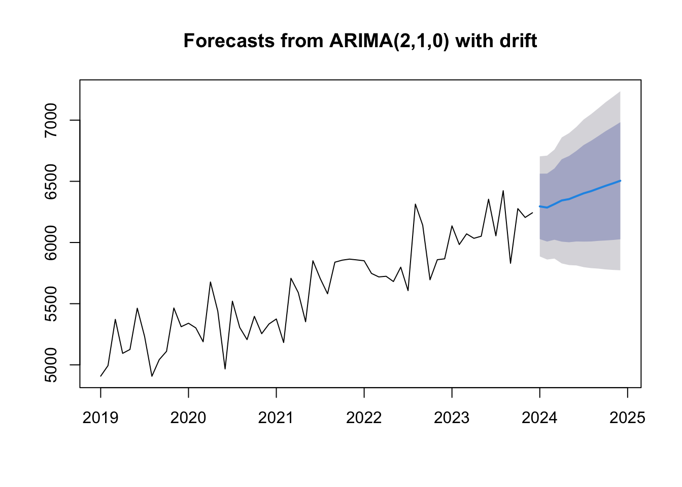
# Use auto.arima to automatically fit an ARIMA modelfit_model <-auto.arima(df$attendance_ts)# Forecast next 12 monthsfuture_forecast <-forecast(fit_model, h =12)# Plot the forecastplot(future_forecast)
In the plot, the blue line shows the forecast for the next 12 months. The shaded region represents the 80% and 95% prediction intervals. You can (hopefully) see why time-series analysis is so useful, and we’ll learn more about time-series analysis in the B1704 Research Methods module.